As a believer in the future of blockchain technology and the need for a global currency I remain committed to this sector. For those that ask why, I offer something I wrote a few years ago:
“In 2008 and 2009, as the financial and banking world was thrown from side to side in a world of uncertainty, I recall some of the most respected people, individuals of great intellect, leaders, those that saw the world through logic that was without panic or undue fear, talking about what we needed to right the ship. Their comments were not about remedies borne from Central Banks pumping liquidity into the system, buying bad debts from banks and other financial entities, and funding government obligations to suppress interest rates. They spoke of the need for technology to emerge, to once again bring about innovation that would change the dynamics of our economies, that would ignite new growth, that would raise the standard of living for a global population, and, in their words, instill the confidence that humankind, that human curiosity, would be the engine that would bring stability, promise, optimism, economic and social growth to a wounded world. I embraced those words, not knowing what the next chapters would bring, but believing that there would be a better tomorrow that was not cobbled together with band-aids and unsustainable one-off remedies. Why were those words so memorable for me? History. History provides the backbone needed to understand and to believe, and it is history that raised those words, those ideas, to the forefront of my mind.
Assembly lines, motorized vehicles, the railroad, the internet, fracking, electricity, the steam engine, the printing press, the telephone, the computer, air travel and the airplane, are all discoveries, forms of innovation, ideas that changed the world. The Blockchain may be, in the context of making new history, the development we write about in the future that freed commerce, that connected economies throughout the world in ways that were never thought possible, that brought the unbanked population into the world of innovation and participation, that took the internet to a new level of integration in life that empowered the individual. I am betting that we are possibly at a junction that strikes fear into the mainstream, those that rely on the comfortable way of doing things, while emboldening those that are explorers and entrepreneurs with the promise of success borne from ideas that feel boundless. The next chapters in time will be driven by the Blockchain and all its implications as it joins with the Internet of Things, Artificial Intelligence, Contract Law, Foreign Exchange, Banking, Commerce, and the fundamental engagement by people in all aspects of being connected together for progress and a better existence than we have known to date.
That is what history tell us. New ideas, birthed from existing practices and understanding, seen through a different lens, changes the path we are on. Progress and the human mind are intertwined, and that is why the global engagement around the Blockchain and the emergent forms of new means of exchange between people are being driven today by the grass roots which embrace progress as the most exciting form of life. There is a growing voice backed by empowering new technology which is changing the world, adding to history, as we try to understand the possibilities of becoming unencumbered by the myriad of middle-men and regulation that stifle economic and social growth. Are you ready for this new adventure, this new chapter? It is scary and exciting, but it is one change I do not want to miss!”
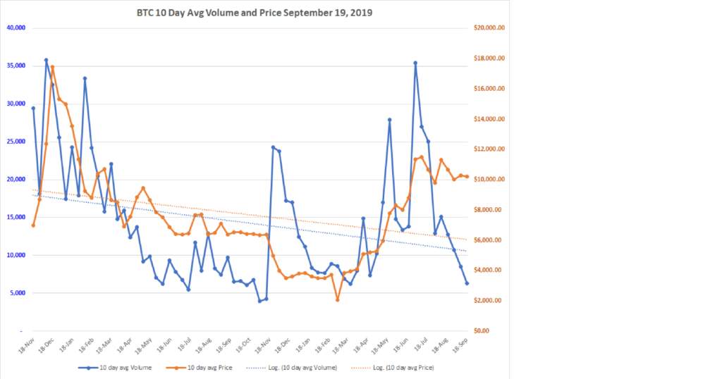
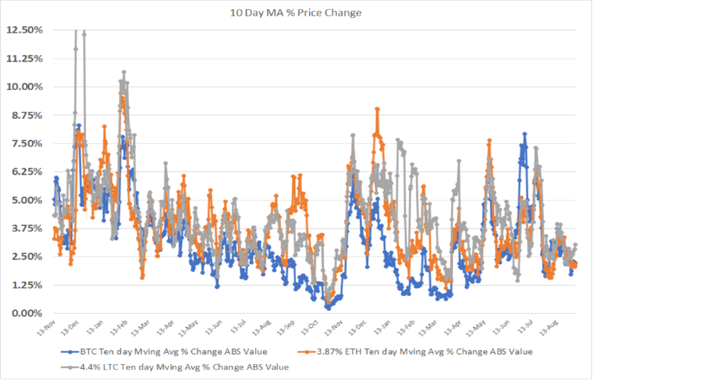
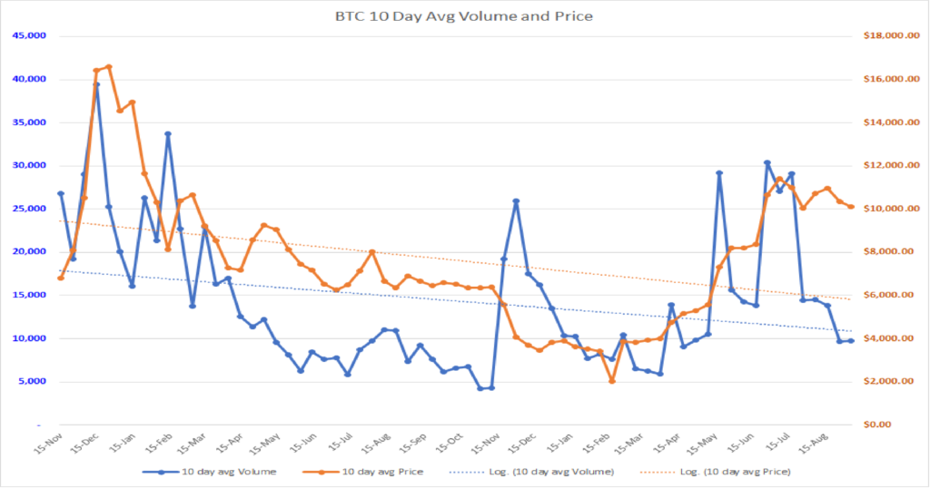
I wrote the above to share with everyone what I feel about the potential promise of the next iteration of the internet, moving from a social/news/commerce communication platform to an empowerment and value platform. While I am no less optimistic about what I see occurring, the Headline above of Hold, Hold, Hold….is meant to indicate that the available data tells me that I should not invest more at this time in Crypto-assets until further signs emerge of greater participation by the people of the world. This is not because of a diminution in my belief of the value that is to be created here, but is about the data informing me of the current market state, a state that reflects strong building underneath but weak participation of the world’s people in owning/using crypto-assets. Growth is present, but it is not viral growth that reveals mass interest and adoption. The price swings are still significant, the volume of crypto-currencies that move each day is static over the longer-term, and the political and financial institutional resistance remains high. Patience is the keyword, along with Hold, Hold, Hold.
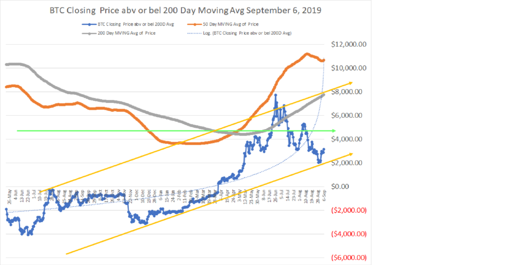
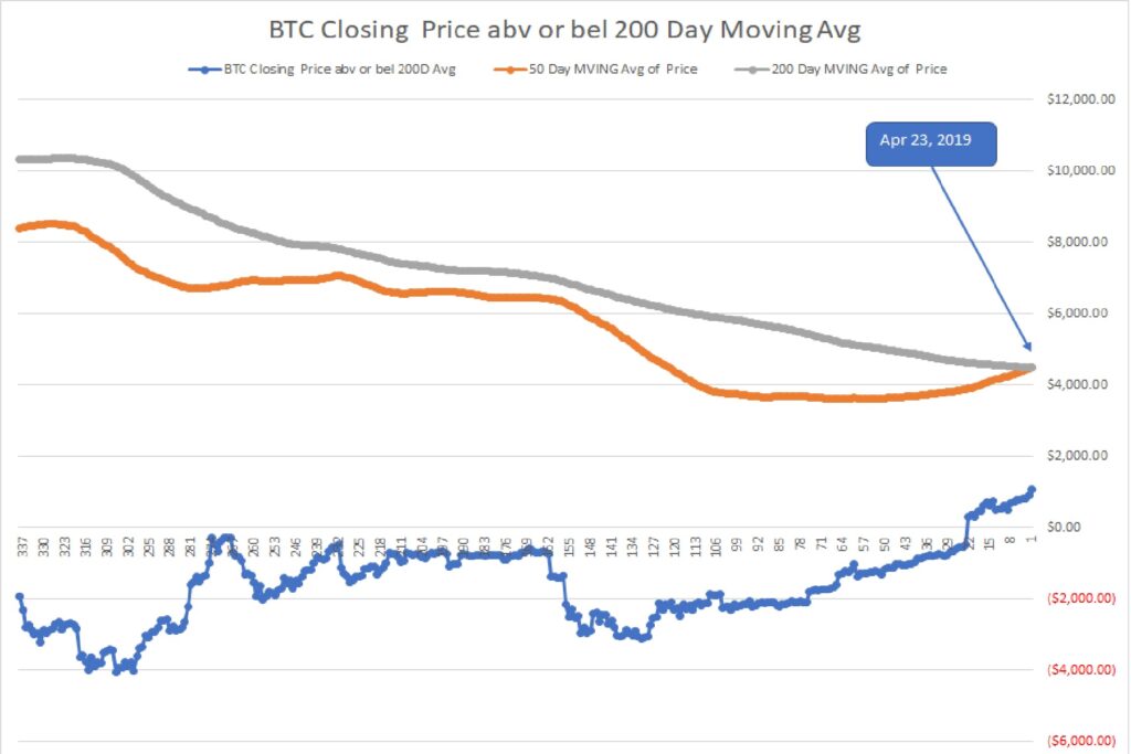
In the menu section of Charts, you will find the latest data on volume and price as of October 4, 2019. I hope they are informative to you and help you in the decisions you may make.
Wishing you all the best,
Tom
The named entities or Blockchains set forth above/below do not represent recommendations to purchase or in any way reflect investment advice. One of the key variables that is critical for deciding to invest is missing. That variable is the current valuation of each token or asset vs the overall market and a reasoned forecast of future performance vs the market. What is presented below attempts to inform and to encourage research, to learn about each, and to come to an opinion of whether any of them or all of them strike you as being an important participant in the future development of digital asset platforms. Charts of technical price levels and movements are presented to educate those unfamiliar with price patterns. These examples of real price activity show how prior price levels may be used to identify market points of price resistance or support. Use this information as you see fit, but it is recommended that you see this as an educational/informative tool only. This information is only part of the array of focus areas needed in making any investment decision, accordingly, it is best to not rely on one type of analysis for your capital allocation decisions.